Overview

This article is all about the fomulation of an important concept arising in computer science, the Transaction. Transaction is usually considered to be a set of operations that maintain the ACID properties, which is an useful abtraction for programmers to write reasonable and effective code. In the past a few decades, various transactional algorithms were invented for achiving efficiency. However, it’s hard to reason about the correctness of a transactional algorithm because of the complex case where multiple transactions executed interleaved.

A proper fomulation of the transaction concept is essential to the correctness of algorithm. In this article, we will build the formulation of transactions in the following order:

The concept of Page model, and the definition of a transaction under this formulated model.
The concept of history and schedules, which is used to describe what is a correct transaction execution.
The syntax and semantics of transactions.

The Computational model

A model is the basis of formulating some concept. Similar to a mathematical theory, where the very basic axioms are presented, the computational model provides certain context and assumption when building the theory of transactions. The preceding theory of transaction are all based on such modle. There are a few steps to define a computational model:

The data or object to manipulate and its associated elementary operations.(i.e. Not divisible)
The definition of a transaction.
Based on the definition of transaction, we define the concept of history and schedule, which describes the execution of multiple transactions
According to the definition of history and schedule, we need to define what is a correct history or schedule in the sense of ACID senmantics.
The algorithm to generate correct history or schedule.

We will only cover the Page model in the first step and not cover the algorithm in the last step, also, in the forth step, there are various kinds of concepts about correct history and we will only cover a few.

Page Model

Data objects and elementary operation

The page model originates from database theory. In traditional database, each operation will eventually be converted into a sequence of operations on a disk page. The page is usually of 4KB size, any read or write to it is considered to be atomic.

We formally define the objects of page model as follows:

$D=\{x, y, z\ldots, \}$

$D$ is a finite set of data items that can be manipulates by transactions. Each data item $x$ provides two kinds of operations: $r(x)$, $w(x)$， which represent reading and writing respectively. Both $r(x)$ and $w(x)$ are atomic (elementary), that means both operations are indivisible and no “smaller” operations can be performed on these data items.

The Definition of transactions

Based on the axioms of data objects described above, we can define transaction in a formular way. In database systems, a transaction is usually a set of operations enclosed by special tokens like “Transaction Start”, “Transaction Commit” and “Transaction Abort”. Operations in the transaction are guaranteed to be executed in ACID manner. Each operation can be pretty complex SQL statement, for example, UPDATE student.score = 5 where student.age > 10.

However, complex operations are converted into a sequence of operations of which each is a page write or read. Thus, a intuitive definition of a transaction is as follows:

A transaction $t$ is a finite sequence of actions as follows:
$t = p_1p_2\ldots p_{n}, \quad n<\infty, p_{i}=r(x)\;\mbox{or}\;w(x), x\in D$

Simply speaking, a transaction is a finite sequence of the atomic operations on pages. However, this definition restricts the transaction only to execute step by step, which may lose parallism. Recall that in a database transaction, operations without dependency relationships can be executed in parallel, the order only matters between operations that have depends on each other. For example, within a tranaction, a SQL statement may read records satisfying specific requirements and then only manipulate these records. This consideration introduces the transaction definition based on partial order:

A transaction $t$ is a set with a partial order $<$ on it. The set consists of read or write operations on data items, that is:
$t = (\mbox{OP}, <),\quad \mbox{OP}=\{op\mid op=r(x)\;\mbox{or}\;op=w(x), x\in D\}$
Also, if $p, q\in \mbox{OP}$ and $p$, $q$ access the same data item and at least one of them is write operation, then $p < q \or q < p$

A partial order on $\mbox{OP}$ is a subset of the cartisian product $\mbox{OP}\times \mbox{OP}$, that satisfies reflexivity, antisemmetry and transitivity. you can simply understand partial order as the execution order between actions, however, this relationship are not guaranteed to exist between any two actions. Two actions without this partial order relationship can be executed in parallel.

The last restriction says that if two operations access the same data item (and if one of them is write) then they must be ordered. This is an obvious constraints: if two operations happens “simoutaneously” on one data item and one is write, the final status of the data item will remain ambiguous.

Further more, the definiton of sequence of actions can be viewed as a special case of partial order definition, that is, the partial order is a total order, thus we can list all contained actions as a sequence.

Semantics of transactions

We have give a strict definition of transaction in the context of page model operations. However, we have not yet clarify what each step is doing. We will describe the semantics of each action.

First consider the sequel case, where transaction is defined as a finite sequence of actions. In this definition, have:

For read operation $p_{j} = r(x)$, its semantic is to read the contents of the object into a local variable:
$v_j := x$
For write operation $p_{j}=w(x)$, its semantic is to first calculate a write value, then write the value into data item $x$. The way to calculate this write value can be describe as a multi-variable function of the value it has previously read:
$x := f(v_{j_1}, v_{j_2},\ldots, v_{j_r})\\ \{j_1, j_2,\ldots, j_r\}=\{j_k\mid p_{j_k} < p_{j} \and p_{j_k} \mbox{is read} \}$

For definition based on partial order, the read operation has the same semantics, however, for write operations, the read happen before a specific write depends on the defined partial order relationship. When define a transaction, the user must specify the partial order clearly.

Transaction Execution

The transaction we defined above is a static concept, it simply presents all operations within a transaction and specify their relationship between each actions. The relation is defined by the user, or the one that creates this transaction. However, to execute transactions, especially concurrent-executing multiple transactions, is a more dynamic and complex process.

There are a few challenges for concurrent transactions execution:

The correctness. Each transaction execution must satisfy ACID property. This is a problem of scheduling: given actions of all transactions, how can you arrange them so that the ACID is satisfied.
Online scheduling. In practice, the system can not wait all transactions arrives, do arrangement on them and then execute them in batch. Instead, the system has to make real-time decision on which transaction should execute, with new incoming transactions.
Efficiency, list all possible arrangements of a batch of transactions could be a naive solution to guarantee correctness, however, it’s inpractical for real world systems.

Anomalies for Transaction Execution

There are a bunch of anomalies when concurrent transactions execute. We list a few archetypical anamalies here, to better clarify the possible issues of concurrent execution and the importance of ACID properties.

Lost update

The lost update problems happens when a transaction’s execution results overwrite another’s results, here is an example:

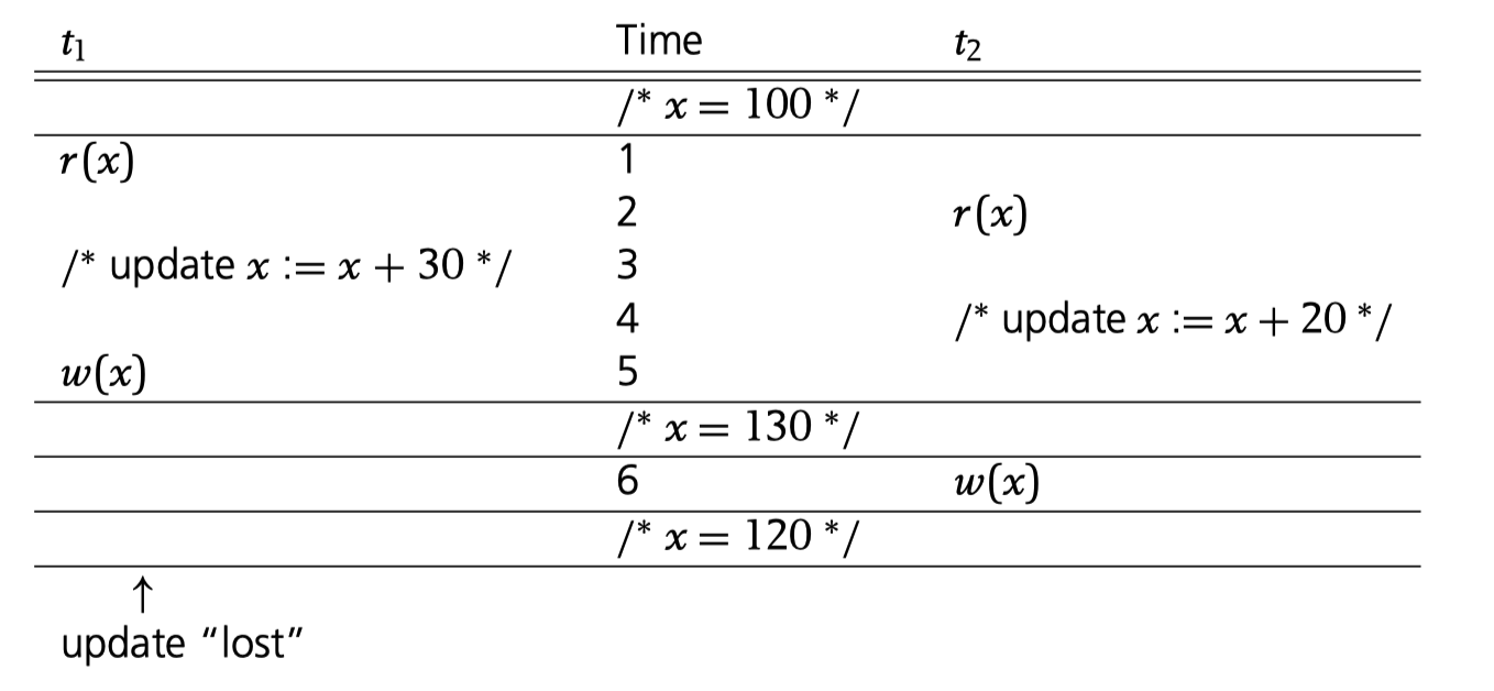
Two transactions wants to update the variable x. However, the results executed by the first transaction is overwritten by then second transaction, causing the final state of the variable to be 120. However, in the ACID view, if two transactions execute successfully, their update should make effect on the variable. That is, the final state of $x$ should be 150.

In-Consistent Read

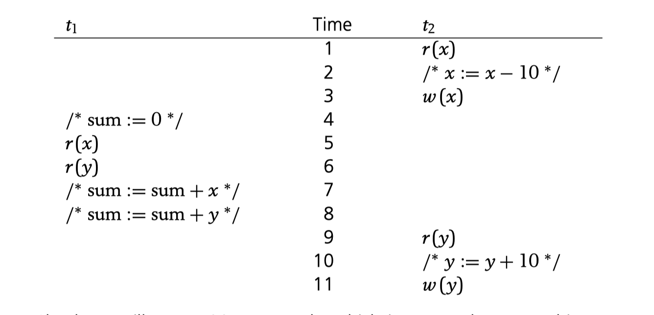
In this example, the transaction t2 aims to maintain an invariable: x+y. That is, before or after the transaction t2 executes, the value $x+y$ should remain constant. Here the value $x+y$ means the value read by another transaction.

However, in the above execution sequence, the transaction t1 would read modified value of $x$ and unmodified value of $y$, causing this invariant false.

Dirty-Read / Read uncommitted

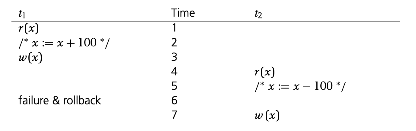
The last anomaly happens when a transaction reads uncommitted data of another transaction. More seriously, tranction $t_2$ reads $t_1$’s uncommitted value $x$ and do some modification based on that read. However, the transaction $t1$ shuts down while the effect of $t2$ based on $t1$ still remains, which is invalid.

The concept about history and schedule

The described anomalies above, reveal challenges to a transactional processing system. The key to the avoid these anomalies is to provide algorithms for generating correct execution schedules. Here we introduce the concept about history, which describes the execution of multiple transactions, and the concept of schedule, which is a prefix of history, that indicates there are some undecided transactions.

History

Simply speaking, a history is an execution arragements of transactions that maintain the dependency relationship of contained transactions. Here is the formal definition:

Let $T = {t{1},\ldots,t{n} }$ be a (ﬁnite) set of transactions, where each $t{i} \in T$ has the form$ t_i = (\mbox{op}{i}, <{i})$, with $\mbox{op}{i}$ denoting the set of operations of $t{i}$ and $<{i}$ denoting their ordering, $1 \leq i\leq n$.

A history for $ T $ is a pair $s = (\mbox{op}(s), <_{s} )$ such that:

$\mbox{op}(s)\subseteq \bigcup{i=1}^{n}\mbox{op}{i}\cup\bigcup{i=1}^{n}{a_i, c_i}$ and $\bigcup{i=1}^{n}\mbox{op}_{i}\subseteq \mbox{op}(s)$ ,i.e., $s$ consists of the union of the operations from the given transactions plus a termination operation, which is either a $c_i$ (commit) or an $a_i$ (abort), for each $t_i \in T$;

$(\forall i, 1\leq i\leq n): c_i\in \mbox{op}(s) \Leftrightarrow a_i\notin \mbox{op}(s)$, i.e., for each transaction, there is either a commit or an abort in $s$, but not both;

$\bigcup{i=1}^{n}<{i}\subseteq <_{s}$ , i.e., all transaction orders are contained</u> in the partial order given by $s$;

$(\forall i, 1 \leq i \leq n)(\forall p \in \mbox{op}i): p <{s} ai\mbox{ or } p <{s} c _i$, i.e., the Commit or Abort operation always appears as the last step of a transaction

Every pair of operations $p, q \in \mbox{op}(s)$ from distinct transactions that access the same data item and have at least one write operation among them is ordered in $s$ in such a way that either $p <{s} q$ or $q <{s} p$.

As we can see, this definition of history is intuitive: operations of all transactions are contained and their individual order are maintained. An additional commit or abort flag is added to the tail of each transaction to mark the end of it.

History is used to describe a complete execution since it contains all operation actions. There are some time we can’t know all actions of all transactions, thus the execution track we give is incomplete, this is called schedule, which is the topic for next section.

Here we have a special case of history, in which all transactions are ordered in some sense:

Serial History: Two transactions $t_i$ and $t_j$ are called ordered in a history $s$, if all operations in $t_i$ are before $t_j$, or vice versa. If any two transactions in history $s$ are ordered, then $s$ is called a serial history.

Examples of history

Here we give an example about history. There are three transactions $t_1, t_2, t_3$, their operations are indiced with their individual transactio id. The orders of operations in each transaction are as follows:

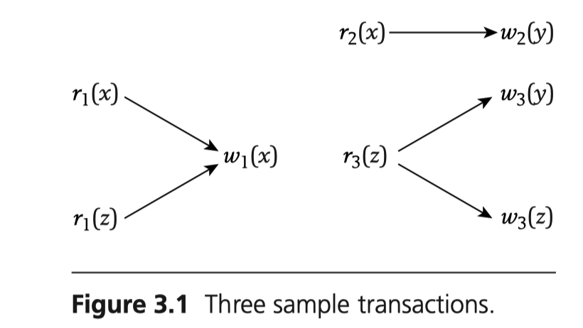
We can give a history of these three transaction execution as follows:

Total order case

$r_1(x)r_2(x)r_1(z)w_1(x)w_2(y)r_3(z)w_3(y)c_1c_2w_3(z)c_3$

This is a history written in total order (which is a special case of partial order). We can check that the sequence contains all operations of all transactions and each transaction is ended with a commit flag. The order within each transaction is maintained, and actions from different transactions that accesses the same data item are ordered as well.

Partial order case

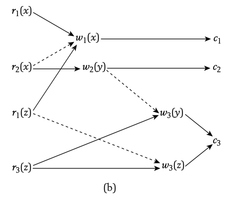
The above picture shows a history in partial order. Except for the existed partial order of each transaction, addtional order is added between transactions when they access the same data item. e.g. $w_2(y)$ and $w_3(y)$, $r_1(z)$ and $w_3(z)$. The additional commit flag is added at the tail.

Though not necessary, we still explicitly state the relationship between the total order case and partial order case. A partial order can be viewed as a DAG (Directed Acylic Graph). And the total order can be constructued using tological sort algorithm.

Schedule

A history is constructed when all actions of all transactions are known to the system. However, this is not a necessarily true assumption, especially for an online transaction scheduler. The system may constantly see incoming transactions and has to decide on which transaction to be executed. That is, we need the system to generate partial execution history.

We introduce the concept about schedule. It’s just a simple definition:

A schedule is a preﬁx of a history.

For a total case, i.e, the history a sequence of actions together will commit or abort flag, the “prefix” is well defined. However, for partial order case where a history is itself a DAG, the “prefix” is not that clear, we give the formal definition of “prefix” in the sense of partial order:

Let $s = (\mbox{op}(s), <{s})$ be a history, i.e, a partial order set. Then a prefix of $s$ is a partial order set $s’=(\mbox{op}(s’), <{s’})$ satisfies:

$\mbox{op}{s’}\subseteq \mbox{op}{s}$

$<{s’}\subseteq <{s}$

$(\forall p\in \mbox{op}(s))(\forall q\in \mbox{op}(s’)): p<{s}q\Rightarrow p\in \mbox{op}{s’}$

$(\forall p,q\in \mbox{op}(s’)): p<{s}q\Rightarrow p<{s’}q$

The prefix of a history based on partial order describes a few paths to an end point. The third axioms says that if an element in the prefix, then any predecessor must also be in the prefix. The second axiom requires the prefix has no additional order compared with original set. The forth axiom requires the order is maintained in the prefix.

Examples of schedule

Total order case

We still uses the examples used above, consider the following history:

$r_1(x)r_2(x)r_1(z)w_1(x)w_2(y)r_3(z)w_3(y)c_1c_2w_3(z)c_3$

Then the following are its prefix, thus schedules:

$\begin{aligned} &r_1 (x)r_2 (x)r_1 (z)w_1 (x)w_2 (y)r_3 (z)w_3 (y),\\ &r_1 (x)r_2 (x)r_1 (z)w_1 (x)w_2 (y),\\ &r_1 (x)r_2 (x)r_1 (z) \end{aligned}$